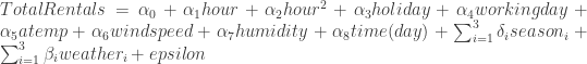
The Kaggle bike sharing competition asks for hourly predictions on the test set, given the training data. The latter consists of the first 19 days of each month, while the test set is the 20th day to the end of each month. As a base model, I’ll just use linear regression. The model is
Here time indicates the day (details later). Sorry for the horrible latex formatting. I’m new to using latex in wordpress and don’t want to spend time right now figuring out how to align equations in wordpress. The variables are
- datetime
- season: Dummy for months 4-6 (2), months 7-9 (3), fall (4). Leave out winter (1)
- holiday: Is the day a holiday?
- working day: Is the day a working day?
- weather [1-3]: Dummy variables for weather
- 1: clear (left out)
- 2: mist, cloudy, broken clouds
- 3: light snow, light rain, thunderstorm
- 4: heavy rain, thunderstorm, snow and fog
- atemp: temp feels like
- humidity
- windspeed
- total rentals
There are several things to note in the model. First, I assume a linear deterministic time trend. In other words, the expected change in count from t to t+1 is constant for all t. There is no acceleration (or deceleration) in trend growth. This assumption is important for the theoretical implications of OLS (in particular consistency and asymptotic normality). Another model would take into account (and check for) stochastic time trends, however I don’t do that here. Second, hour is included with its squared term. Why? Its reasonable to expect that the impact on rentals from hour of the day starts low, increases toward mid day and then decreases at night. The squared term allows for parabola opening downward, which could depict this situation. Higher orders of hour could be included to fit more complex functional relationships. Perhaps there are different peaks for morning… afternoon… evening… etc. This model uses the second order to capture the overall trend (again I expect to see an inverted parabola in hours). Third, dummy variables are created for the season and weather variables. One type for each category must be left out to avoid perfect multicollinearity.
I’ll be extending the R code from the previous two posts on kaggle bike sharing. First create the time variable. I need to be a little careful here because of the missing data. Suppose I start numbering each day in the training set, starting with January 1st 2012 as 1. January 19th would be 19, but then the 20th day is missing (as it is in the test set). February 1st should be 19 + however many days are left in January. The following code creates this time variable and runs the regression stated above.

The regression output for this model is

The p value for the test statistic is small enough so that the model is not useless. Formally I can reject at the one percent level that all coefficients are not simultaneously zero. Lets look at some of the coefficients for a minute. As expected, the hour variable forms an inverted parabola with maximum at hour 14.63 (shortly after 2:30PM). In words, starting at midnight, increasing hours increases total demand until around 2:30PM, wheres increasing the hour after decreases total demand. Higher feels like temp corresponds to higher total rentals, while higher humidity corresponds to less rentals. It may have been interesting here to add a non linear (squared) feels like temp variable to capture since too hot could correspond to less rentals (again we would expect an inverted parabola in feels like temp).
The season and weather estimates give some counter intuitive results. First, all else equal months 1-3 and 10-12 raise rentals from winter time levels. Months 7-9 however decrease rentals. Intuitively I expect all of them to be positive. The second counter intuitive result is that when compared to the best weather, the worst weather reduces rentals by less than better weather. Again, very hard to explain. Could the kaggle coding for weather be wrong? The kaggle stated season indicators didn’t match up, so maybe the weather indicators are off too.
The following code generates a predicted vs. observed plot aggregated by day.

And corresponding plot

